Lecture 10 Double Integrals and Double Integrals Over Rectangles

Text References: Course notes pp. 37-52 & Rogawski 14.8, 15.1-15.2

10.1 Recap

Last time, learned how to apply the Method of Lagrange to find the extrema of a function \(f(x,y)\) subject to a constraint \(g(x,y)=K\).

Exercise 10.1 Consider the level curves of a function \(f (x, y)\) and the constraint curve \(g(x, y) = k\) (in red). Estimate the maximum and minimum values of \(f\) with constraint \(g(x, y) = k\).

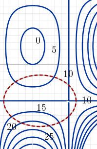
Figure 10.1: Level curves of an unknown function and constraint curve \(g(x,y)=K\)

Solution. We check which level curves intersect with the constraint curve. We estimate that the maximum value is approximately \(24\) (between \(20\) and \(25\), but closer to \(25\) and the minimum value is approximately \(2\) (between \(0\) and \(5\), around halfway in between).

10.2 Learning Objectives

• Given a function of several variables, integrate it with respect to a chosen variable.
• Evaluate iterated integrals over rectangular domains

10.3 Partial Integration

In the past few weeks, we’ve been working on generalizing ideas from differential calculus; now, we’re going to focus on integral calculus for a little bit.

Just like partial differentiation, we have a concept of partial integration: we can take the partial integral of a function of several variables by treating the variable of integration normally and any other variables as constants. The differential tells us which variable is the variable of integration.

Exercise 10.2 Calculate \(\displaystyle \int (2x+3y^2)dy\).

Solution. The differential is \(dy\), which means that \(y\) is the variable of integration. Treating \(x\) as a constant, we get \[\displaystyle \int (2x+3y^2)dy = 2xy + y^3 + g(x)\]

Note that instead of a constant \(C\), we have a function \(g(x)\): since our variable of integration is \(y\), any function of \(x\) will disappear when we take the partial derivative with respect to \(y\).

Partial integration can help us identify a function (up to a constant) if we know its partial derivatives.

Exercise 10.3 Find \(f(x,y)\) up to a constant if \(f_{x}(x,y)=4x^3y^3+3y^2+1\) and \(f_y = 3x^4y^2+6xy\).

Solution. Using partial integration, we have \[f(x,y)=\displaystyle \int f_xdx = \int (4x^3y^3+3y^2+1) dx =x^4y^3+3xy^2+x+g(y)\] and also \[f(x,y)=\displaystyle \int f_ydy = \int (3x^4y^2+6x)y dy = x^4y^3+3xy^2+h(x)\]

Putting it all together, we have \[f(x,y)=x^4y^3+3xy^2+x+g(y) \quad \mbox{and} \quad f(x,y)=x^4y^3+3xy^2+h(x)\]

Since the expressions are equal, this implies that \(x+g(y)=h(x)\); it must be that \(g(y)=C\) for some constant \(C\). Therefore, \(f(x,y)=x^4y^3+3xy^2+x+C\).

10.4 Double Integrals

Until now, we’ve been doing a form of antidifferentiation; now, we’re going to work on defining double integrals.

To start, we’ll assume that the domain of integration is rectangular, that is, \(a\leq x\leq b\) and \(c\leq y\leq d\), and that \(f>0\) everywhere in this domain.

We can partition the region along the \(x\)-axis into \(m\) intervals of length \(\Delta x=\frac{(b-a)}{m}\); likewise, we can partition the region along the \(y\)-axis into \(n\) intervals of length \(\Delta y = \frac{(d-c)}{n}\). We’ve now partitioned the domain into rectangles with area \(\Delta A=\Delta x\Delta y\).

In each rectangle, we choose a point \((x_i^*, y_j^*)\). Then \(f(x_i^*, y_j^*)\Delta A\) represents the volume below the surface \(z=f(x,y)\) over the rectangle. Summing all of these volumes gives us an approximation of the volume below the surface over the domain. We also expect that as \(\Delta A\to 0\), the error in the approximation of the volume should approach zero. This motivates the following definition:

Definition 10.1 The double integral of a continuous function \(f(x,y)\) over a rectangular region \(R\in \mathbb{R}^2\) is \[\displaystyle \int_R f(x,y)dA =\lim_{m, n \to \infty}\sum_{i=1}^m\sum_{j=1}^nf(x_i^*, y_j^*)\Delta A\]

This interactive applet gives some intuition for what’s happening in 3D space.

10.5 Double Integrals Over Rectangles

Rectangles are particularly nice domains over which to integrate: we can evaluate such integrals by performing partial integration of one variable at a time. The intuition for this is that when we fix one of the variables, we are singling out the cross-section of \(z=f(x,y)\) along that constant plane and calculating the area below this curve. Now, sweeping along the other variable, we give our cross-section slice some thickness and create a volume. A more detailed explanation of this can be found in the course notes.

From this intuition, we get the following result: If \(R=[a,b]\times[c,d]\), then \[\displaystyle \int_R f(x,y) dA=\int_c^d \int_a^b f(x,y) dx dy = \int_a^b \int_c^d f(x,y) dy dx\]

Notice that for these types of integrals, the order of integration doesn’t matter! Unfortunately, this isn’t always the case; it’s one of the reasons we like integrating over rectangles so much. Given that the order of integration doesn’t matter, this gives us a bit of freedom in deciding which order of integration works best.

Another nice property of integrals over rectangles is that if the integrand can be factored into a function of \(x\) and a function of \(y\), then the entire integral can be factored into an integral in \(x\) and an integral in \(y\). More formally, suppose that \(f(x,y)=g(x)h(y)\), then \[\displaystyle \int_c^d\int_a^b f(x,y) dxdy = \displaystyle \int_c^d\int_a^b g(x)h(y) dxdy=\displaystyle \int_c^dh(y)dy\int_a^b g(x) dx\]

Exercise 10.4 Evaluate \(\displaystyle \int_2^4 \int_1^9 ye^x dy dx\).

Solution. Note that we first integrate with respect to \(y\) and the with respect to \(x\): \[\begin{align*} \displaystyle \int_2^4 \int_1^9 ye^x dy dx & = \int_2^4 \left ( \int_1^9 ye^x dy \right )dx\\ &= \int_2^4 \left (e^x\int_1^9 y dy\right ) dx\\ &= \int_2^4 \left ( \dfrac{e^xy^2}{2}\right |_{y=1}^9 dx\\ &= \int_2^4 40e^x dx\\ &= 40(e^4-e^2) \end{align*}\]

Exercise 10.5 Evaluate \(\displaystyle \int_0^{1}\int_{-\pi}^{\pi}x\sin(xy)dx dy\).

Solution. We notice that in this case, it’s much, much simpler to integrate first with respect to \(y\), then with respect to \(x\): \[\begin{align*} \displaystyle \int_0^1\int_{-\pi}^{\pi}x\sin(xy)dx dy & = \displaystyle \int_{-\pi}^{\pi}\int_{0}^1x\sin(xy)dy dx\\ & = \displaystyle \int_{-\pi}^{\pi} \left (x \int_0^1 \sin(xy)dy \right)dx \\ & = \displaystyle \int_{-\pi}^{\pi} \left (\dfrac{-x\cos(xy)}{x} \right|_{y=0}^1 dx \\ & = \displaystyle \int_{-\pi}^{\pi} -\cos(x)+\cos(0) dx \\ &= \left . -\sin(x) \right |_{x=-\pi}^{\pi}+ \left. x\cos(0) \right|_{x=-\pi}^{\pi}\\ &= 2\pi \end{align*}\]