Lecture 8 Unconstrained Optimization
Text References: Course notes pp. 26-37 & Rogawski 14.5-14.7
8.1 Recap
Last time, we learned how to compute the gradient of a multivariate function and how to use it to compute directional derivatives.
Exercise 8.1 The surface of a hill is modeled by \(z = 25 - 2x^2 - 4y^2\) . When a hiker reaches the point \((1, 1, 19)\), it begins to rain. They decide to descend the hill by the most rapid way. Which vector points in the direction in which they start their descent?
Solution. We have \(\nabla f (x,y)= \left (-4x, -8y\right)\) and so \(\nabla f (1,1)= (-4, -8)\). This tells us that the largest increase in the rate of change of \(f\) at the point \((1,1,19)\) is in the direction of \((-4,-8)\); to get the direction of the largest decrease, we must go in the opposite direction of \((4,8)\).
8.2 Learning Objectives
- Given a function of several variables, find its critical points.
- Given a function of several variables, use the second derivative test to classify its extrema as local minima, maxima, or saddle points
8.3 Critical Points
As in single-variable calculus, we are often interested in finding the maxima and minima for functions of several variables. Let’s start by defining them.
Definition 8.1 A function \(f(x,y)\) has a local maximum at \((x_0, y_0)\) if \(f(x_0, y_0)\geq f(x,y)\) for all \((x,y)\) in some disc centred at \((x_0, y_0)\).
Definition 8.2 A function \(f(x,y)\) has a local minimum at \((x_0, y_0)\) if \(f(x_0, y_0)\leq f(x,y)\) for all \((x,y)\) in some disc centred at \((x_0, y_0)\).
The idea here is that we should be able to find a disc small enough so that the inequalities hold throughout.
Finding local maxima and minima proceeds in a similar way as single-variable calculus. We know that maxima/minima should only occur at points where the tangent plane is horizontal or at points where the tangent plane can’t be defined.
The tangent plane is horizontal when \(\nabla f = \vec{0}\), which motivates the following definition:
Definition 8.3 A point \((a,b)\) in the domain of \(f(x,y)\) is a critical point if either
- both \(f_x\) and \(f_y\) are zero; or
- at least one of \(f_x\), \(f_y\) is undefined
Just like in single-variable calculus, not all critical points are extrema; critical points which are neither maxima nor minima are called saddle points.
Exercise 8.2 Find the critical points of \(f(x,y)= x^3-4x^2+4x-4xy^2\).
Solution. The critical points are those were \(f_x(x,y)=0\) and \(f_y(x,y)=0\). In this (and most) cases, the tangent plane of this function is defined everywhere.
We have \[f_x(x,y) = 3x^2-8x+4-4y^2 \quad \mbox{(1)} \quad \mbox{and} \quad f_y(x,y)= -8xy \quad \mbox{(2)}\] Setting \(f_x(x,y)=0\) and \(f_y(x,y)=0\), from \((2)\) we get that either \(x=0\) or \(y=0\)
- If \(x=0\), then from \((1)\) we get that \(4-4y^2=0\) and so \(y=\pm 1\). We get the critical points \((0,-1)\) and \((0,1)\).
- If \(y=0\), then from \((1)\) we get that \(3x^2-8x+4=(3x-2)(x-2)=0\) and so \(x=2/3\) or \(x=2\). We get the critical points \((2/3, 0)\) and \((2,0)\).
The function therefore has four critical points: \((0,-1)\), \((0,1)\), \((2/3, 0)\), and \((2,0)\).
8.4 The Second Derivative Test
Now that we know how to find the critical points of a function, the next step is to classify each of them as a maximum, a minimum, or a saddle point. In single-variable calculus, we relied on the sign of the second derivative to help us; now, we rely on the set of second partial derivatives in what’s known as the Second Derivative Test.
Theorem 8.1 Let \((a,b)\) be a critical point of a function \(f(x,y)\) and suppose that the second-order partial derivatives of \(f\) are continuous in some neighbourhood of \((a,b)\). Let \(D(x,y)=f_{xx}f_{yy}-(f_{xy})^2.\)
- If \(D(a,b) > 0\), then \(f\) has an extremum at \((a,b)\).
- If \(f_{xx}(a,b)< 0\), then the extremum is a maximum
- If \(f_{xx}(a,b)> 0\), then the extremum is a minimum
- If \(D(a,b)< 0\), then \(f\) does not have an extremum at \((a,b)\), i.e., \((a,b)\) is a saddle point
- If \(D(a,b)= 0\), then the test is inconclusive.
One useful way to think about this test is by using matrices. If we consider the matrix \[Hf(x,y)=\begin{bmatrix}f_{xx}(x,y) & f_{xy}(x,y)\\f_{xy}(x,y) & f_{yy}(x,y)\end{bmatrix}\] then \(D(x,y)\) is the determinant of this matrix, which is called the Hessian matrix.
Exercise 8.3 Classify the critical points of \(f(x,y)= x^3-4x^2+4x-4xy^2\) as maxima, minima, or saddle points.
Solution. We have
- \(f_{xx}(x,y)=6x-8\)
- \(f_{xy}(x,y)=-8y\)
- \(f_{yy}(x,y)=-8x\)
Therefore \(Hf(x,y)=\begin{bmatrix} 6x-8 & -8y\\-8y & -8x\end{bmatrix}\) and has determinant \(D(x,y)=-48x^2+64x-64y^2\) From the previous exercise, we found that the critical points of the function are \((0,-1)\), \((0,1)\), \((2/3, 0)\), and \((2,0)\).
- \(D(0,-1)=-64 <0\) so \((0,-1)\) is a saddle point.
- \(D(0,1))=-64 <0\) so \((0, 1)\) is a saddle point.
- \(D(2/3,0)=64/3 >0\) and \(f{xx}(2/3,0)=-4<0\) so \((2/3,0)\) is a maximum.
- \(D(2,0))=-64 <0\) so \((2, 0)\) is a saddle point.
Use the interactive applet to see what’s happening in 3D space.
8.5 Local Extrema and Level Curves
Knowing the local extrema of a function can be very helpful in both graphing the function and plotting its level curves. We make two important observations:
- In the neighbourhood of a local maximum or minimum, the level curves will (roughly) be concentric circles or ellipses.
- In the neighbourhood of a saddle point, one level curve will cross over itself.
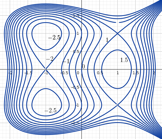
Figure 8.1: Level curves of an unknown function
Solution. The graph suggests that the function has six critical points.
- We conclude that \((-1,1)\) and \((-1,-1)\) are local minimum points since the values of \(f\) appear to decrease as we approach these points from all possible directions.
- We conclude that \((0,1)\) is a local maximum point since the values of \(f\) appear to increase as we approach this point from all possible directions.
- We conclude that \((-1,0)\), \((1,1)\), and \((1,-1)\) are saddle points since the values of \(f\) can increase or decrease as we approach these points depending on the direction we choose. For example, if we approach point \((-1,0)\) from below, then the function values appear to decrease from \(1.5\) to \(1\), but if we approach from the left, then the function values appear to increase from \(0\) to \(1\).