Lecture 4 Tangent Planes, Linear Approximation and Differentials
Text References: Course notes pp. 10-22 & Rogawski 14.4, 11.1, 14.6
4.1 Recap
Last time, we learned how to calculate first and higher-order partial derivatives of functions. As we’ll learn, partial derivatives are key to helping us calculate tangent planes and linear approximations.
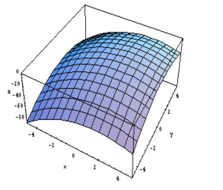
Exercise 4.1 At which point above the \(xy\)-plane will both partial derivatives be positive?
- \((-5, -5)\)
- \((5, -5)\)
- \((5, 5)\)
- \((-5, 5)\)

Solution. The answer is a. At this point, both tangent lines (along the \(x\) and \(y\) directions) have a positive slope. In other words, the surface is moving upward in both the \(x\) and \(y\) directions at this point.
4.2 Learning Objectives
- Given a surface and a point, find the tangent plane to the surface at the point.
- Given a multivariable function, find its linear approximation and use it to approximate the value of the function at a given point.
- Use the differential to calculate change with respect to a given variable.
4.3 Tangent Planes
In single-variable calculus, we learned about the linear approximation to a function. Given a curve \(y=f(x)\) at a point \((x_0, f(x_0))\), the linear approximation of \(f\) at \(x_0\) is given by \(L_{x_0}=f(x_0)+f'(x_0)(x-x_0)\). Our next task is to generalize this to multivariate functions. Our first observation is that for surfaces of the form \(z=f(x,y)\), we will get a tangent plane rather than a tangent line.
Let’s think for a moment about the partial derivatives of a function. Given a point \((x_0,y_0)\), \(f_x(x_0,y_0)\) gives the slope of the tangent line to the cross-section \(y=y_0\) (remember, we’re holding \(y\) as a constant to calculate the partial derivative w.r.t \(x\)) and \(f_y(x_0, y_0)\) gives the slope of the cross-section \(x=x_0\).
From a derivation in your course notes, a non-vertical plane passing through the point \((x_0, y_0, z_0)\) will have equation \[z=z_0+A(x-x_0)+B(y-y_0)\] where \(A\) and \(B\) are constants.
Setting \(y=y_0\), we have \(z=z_0+A(x-x_0)\). Note that we are on the cross-section \(y=y_0\), which we know to have slope equal to \(f_x(x_0, y_0)\). This means that \(A=f_x(x_0,y_0)\). We make a similar argument to find that \(B=f_y(x_0,y_0)\) and therefore the equation of the tangent plane is \[z=z_0+f_x(x_0, y_0)(x-x_0)+f_y(x_0, y_0)(y-y_0)\]
Exercise 4.2 Find the equation of the tangent plane to the surface \(z=\sqrt{x^2+y^2}\) at the point \((3, -4)\).
Solution. We have \(x_0=3, y_0=-4\), and \(z_0=f(x_0,y_0)=\sqrt{3^2+(-4)^2}=5\).
Furthermore, \(f_x = \dfrac{x}{\sqrt{x^2+y^2}}\) and\(f_y = \dfrac{y}{\sqrt{x^2+y^2}}\). Evaluating at the point \((3, 4)\), we have \(f_x(3,4)=\frac{3}{5}\) and \(f_y(3, -4)=-\frac{4}{5}\).
Putting everything together, we find that the tangent plane at point \((3,-4)\) has equation \[z=5+\frac{3}{5}(x-3)-\frac{4}{5}(y+4)\]
4.4 Linear Approximation
We often use the equation of the tangent plane to approximate values of a given function. As long as we’re close enough to the point \((x_0, y_0)\), we can approximate the value of \(f(x,y)\) at a nearby point: \[f(x,y)\approx f(x_0,y_0)+f_x(x_0, y_0)(x-x_0)+f_y(x_0, y_0)(y-y_0)\]
Exercise 4.3 Approximate the value of \(f(x,y)=\sqrt{x^2+y^2}\) at the point \((3.01, -3.99)\)
Solution. Using the linear approximation we found earlier, we have \[\begin{align*} f(x,y) & \approx 5+\frac{3}{5}(x-3)-\frac{4}{5}(y+4) \\ & \approx 5+\frac{3}{5}(3.01-3)-\frac{4}{5}(-3.99+4)\\ & \approx 4.998 \end{align*}\]
Note that this is quite close to the actual value of \(4.99802\)!
4.5 Differentials
When working with linear approximations, it’s common to use differential notation by setting \(\Delta x = x-x_0\), \(\Delta y = y- y_0\), and \(\Delta f = f(x,y)-f(x_0, y_0)\). In this case, we can rewrite the linear approximation as \[\Delta f = f_x(x_0, y_0)\Delta x + f_y(x_0, y_0) \Delta y\]
Notice that the closer we get to the point \((x_0, y_0)\), that is, as \(\Delta x \to 0\) and \(\Delta y \to 0\), the more accurate our approximation. It’s therefore common to replace the \(\Delta\) symbols with \(d\)-notation and the \(\approx\) with an equal sign to get an even more compact expression \[df = f_x dx+f_y dy\] Keep in mind, however, that the point \((x_0, y_0)\) is still playing a role here.
Let’s see how the notation of differentials can be useful.
Exercise 4.4 An isosceles triangle has base \(4\)m and equal angles of \(\frac{\pi}{4}\). How sensitive is the triangle’s area to small variations in the length of the base and the equal angles?
Solution. Note that the height of an isosceles triangle like the one described in this exercise is given by \(\frac{b}{2}\tan(\theta)\). Therefore, the area of the triangle is given by \(A(b, \theta)= \frac{b^2 \tan(\theta)}{4}\).
The differential at \((4, \pi/4)\) is \(dA= \dfrac{\partial A}{\partial b}db + \dfrac{\partial A}{\partial \theta}d\theta\). Calculating the partial derivatives, we find that the change in areas is approximately \[\begin{align*} dA &= \frac{\tan(\pi/4)}{2}db + 4 \sec^2(\pi/4)d\theta\\ &= db + 8 d\theta \end{align*}\]
Therefore the area of the triangle is \(8\) times more sensitive to changes in the equal angles compared to changes in the length of its base.