Lecture 13 The Change of Variable Formula
Text References: Course notes pp. 53-65 & Rogawski 11.3, 15.4-15.6
13.1 Recap
Last time, we learned another technique for solving double integrals: changing to polar coordinates.
Exercise 13.1 Transform the integral \(\displaystyle \int_{-3}^0\int_{-\sqrt{9-y^2}}^{\sqrt{9-y^2}} 1~dxdy\) to polar coordinates (no need to solve the integral).
Solution. We are working with the inequalities \(-3\leq y\leq 0\) and \(-\sqrt{9-y^2}\leq x\leq \sqrt{9-y^2}\). We can rewrite the second inequality as \(x^2=9-y^2 \implies x^2+y^2=9\), which describes a circle of radius \(3\). The additional conditions on \(y\) mean that we are only considering the bottom half of the circle.
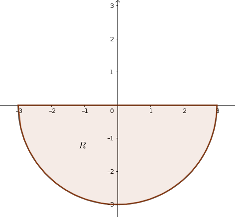
Figure 13.1: Domain of integration
Thus, \(0\leq \rho \leq 3\) and \(\pi\leq\phi\leq 2\pi\). Remembering the factor of \(\rho\) in the integrand, we get \[\int_{0}^3\int_{\pi}^{2\pi}\rho~d\rho d\phi\]
13.2 Learning Objectives
- Evaluate integrals using the change of variables formula.
13.3 Transformations
Thinking back to our work with polar coordinates, we’ve seen that changing coordinates is in fact a transformation which maps the \(xy\)-plane to the \(\rho\phi\)-plane. This is the idea we’re going to try go generalize to help us solve integration problems: if the region of integration is not “nice,” we can apply a transformation to it and turn it into a “nice” region that’s easier to integrate over.
Let’s think for a moment about which regions are particularly nice to integrate over: rectangles! Our goal in coming up with transformations will generally be to transform integrals over non-rectangular domains into integrals over rectangular domains (or, if that’s not so straightforward, into regions of Type I or Type II). As with polar coordinates, we will have to think carefully about what the new area element \(dA\) should be.
Exercise 13.2 Find a mapping which transforms the region \(R_{xy}\) in the first quadrant bounded by the hyperbolae \(xy=1\), \(xy=3\), \(x^2-y^2=2\), \(x^2-y^2=4\) into a square in the \(uv\)-plane.
Solution. Take \(u(x,y)=xy\) and \(v(x,y)=x^2-y^2\). The boundaries of the region will map to the horizontal lines \(u=1\) and \(u=3\) and to the vertical lines \(v=2\) and \(v=4\) in the \(uv\)-plane.
13.4 The Change of Variables Formula
Let’s dive into the main result.
Theorem 13.1 Suppose that the variables \(x\) and \(y\) are related to the variables \(u\) and \(v\) by the equations \(x=x(u,v)\), \(y=y(u,v)\). Then, \[\iint_{R_{xy}}f(x,y)~dxdy = \iint_{R_{uv}}f(x(u,v), y(u,v)) \left |\dfrac{\partial(x,y)}{\partial (u,v)}\right|~dudv\] where \[\dfrac{\partial(x,y)}{\partial (u,v)}=\det\begin{bmatrix}\frac{\partial x}{\partial u}&\frac{\partial x}{\partial v}\\ \frac{\partial y}{\partial u}& \frac{\partial y}{\partial v}\end{bmatrix}\] This function is called the Jacobian of the transformation, and is also denoted by \(J\). Note that \(\left |\dfrac{\partial(x,y)}{\partial (u,v)}\right|\) is the absolute value of the determinant of the matrix of partial derivatives.
When applying the change of variables formula, it’s important to keep a few things in mind:
- The transformation \((x,y)\to (u,v)\) must be invertible on the domain of integration. In other words, we can’t have \(J=0\) at any point on the interior of \(R_{uv}\); we don’t want to lose information by, for example, contracting a line to a point.
- The Jacobian can be understood as area scaling factor of a given transformation. That is, the Jacobian describes the extent to which the associated mapping increases or decreases areas.
- As we might expect, \(\dfrac{\partial(x,y)}{\partial(u,v)}=\dfrac{1}{\frac{\partial(u,v)}{\partial(x,y)}}\)
Exercise 13.3 Evaluate \(\displaystyle \iint_R x dA\) where \(R\) is the region in the first and fourth quadrants bounded by the curves \(y+x^2=0\), \(y+x^2=1\), \(y-x^2=0\), and \(y-x^2=-1\).
Solution. We start by defining a map that converts this region into the unit square in the \(uv\)-plane by setting \(u(x,y)=x+y^2\) and \(v(x,y)=y-x^2\).
Writing \(x\) and \(y\) in terms of \(u\) and \(v\), we can sum \(u\) and \(v\) to find \(y=\frac{u+v}{2}\); and we can subtract \(u\) and \(v\) to find \(x=\sqrt{\frac{u-v}{2}}\). Note that we have \(0\leq u\leq 1\) and \(0\leq v\leq 1\).
Next, we calculate the Jacobian: \[\dfrac{\partial(x,y)}{\partial (u,v)}=\det\begin{bmatrix}\frac{\partial x}{\partial u}&\frac{\partial x}{\partial v}\\ \frac{\partial y}{\partial u}& \frac{\partial y}{\partial v}\end{bmatrix} = \begin{bmatrix}\frac{1}{2\sqrt{2u-2v}}& -\frac{1}{2\sqrt{2u-2v}}\\ \frac{1}{2} & \frac{1}{2}\end{bmatrix} = \dfrac{1}{2\sqrt{2u-2v}}\]
Now, we express the integrand in terms of the new variables: \(x=\sqrt{\frac{u-v}{2}}\).
Putting everything together, we apply the change of variables: \[ \iint_R x dA = \int_0^1\int_0^1 \frac{1}{2\sqrt{2u-2v}}\sqrt{\frac{u-v}{2}}du dv = \int_0^1\int_0^1 \frac{1}{4} du dv = \frac{1}{4}\]
Exercise 13.4 Evaluate \(\displaystyle \iint_R (x^2-xy -y^2) dA\) where \(R\) is the region in the first quadrant bounded by the hyperbolae \(xy=1\), \(xy=3\), \(x^2-y^2=2\), \(x^2-y^2=4\) into a square in the \(uv\)-plane.
Solution. Using the transformation we found in an earlier example, we have \(u(x,y)=xy\) and \(v(x,y)=x^2-y^2\). Note that in this case, writing \(x\) and \(y\) in terms of \(u\) and \(v\) is not so simple; we will use the property of the Jabobian that \(\dfrac{\partial(x,y)}{\partial(u,v)}=\dfrac{1}{\frac{\partial(u,v)}{\partial(x,y)}}\).
\[\frac{\partial(u,v)}{\partial(x,y)} = \det \begin{bmatrix}\frac{\partial u}{\partial x}&\frac{\partial u}{\partial y}\\ \frac{\partial v}{\partial x}& \frac{\partial v}{\partial y}\end{bmatrix}=\det\begin{bmatrix}y & x\\2x& -2y\end{bmatrix}=-2y^2-2x^2\]
and so \[\dfrac{\partial(x,y)}{\partial(u,v)}=\dfrac{1}{\frac{\partial(u,v)}{\partial(x,y)}} = \frac{1}{-2y^2-2x^2}\]
Expressing the integrand in terms of the new variables, we get \[x^2-xy -y^2 = v-u\]