Lecture 19 Interpolating Polynomials

Text References: Course notes pp. 75-100 & Rogawski 4.8, 10.7

19.1 Recap

Last time, we learned about Newton’s Method and how to apply it to find roots of a function.

Exercise 19.1 Consider the following questions:

How many iterations of Newton’s Method are required to compute a root if \(f\) is a linear function?
What happens in Newton’s Method if your initial guess happens to be a root of \(f\)?
What happens in Newton’s Method if your initial guess happens to be a local min or max of \(f\)?

Solution. We have:

Only one iteration is required; the function is equal to its linear approximation.
The iterates will all be equal to the initial guess \(x_0\).
The method will fail since \(f'(x)=0\) at local maxima and local minima.

19.2 Learning Objectives

Use polynomial interpolation to find the polynomial of degree \(n\) which passes through a set of \(n+1\) points \((x_0,y_0), \ldots, (x_n,y_n)\).

19.3 Polynomial Interpolation

Suppose that we are given a set of \(n+1\) points \((x_0,y_0), \ldots, (x_n,y_n))\) and are asked to find a smooth curve which passes through all of them. The simplest curve that can achieve this is a polynomial of degree \(n\), that is, of the form \(y=a_0+a_x1+a_2x^2+\cdots+a_nx^n\).

This interactive applet gives an idea of what we’re trying to achieve:

The question we are now working on is how to find the equation of the polynomial passing through \((x_0,y_0), \ldots, (x_n,y_n))\).

19.3.1 Integer Nodes

Let’s start by considering the simpler case where the values of \(x_0, y_0, x_1, y_1,\ldots\) are integers.

Suppose that we are looking for a degree \(3\) polynomial passing through the points \((0,y_0), (1, y_1), (2,y_2)\), and \((3,y_3)\).

We are looking for a cubic function \(y= a+bx+cx^2+dx^3\); plugging in our points gives

\[\begin{align*} y_0 &= a \\ y_1 &= a+b+c+d\\ y_2 &= a+ 2b+4c+8d \\ y_3 &= a+3b+9c+27d \end{align*}\]

Now, let’s introduce some new notation. The first finite differences are \(\Delta y_n = y_{n+1}-y_n\)

Exercise 19.2 Calculate the first finite differences for the system above.

Solution. We have

\[\begin{align*} \Delta y_0 &= y_1-y_0 = b+c+d \\ \Delta y_1 &= y_2-y_1 = b+3c+7d \\ \Delta y_2 &= y_3-y_1 = b+5c+19d \\ \end{align*}\]

Notice that all of the \(a\)s have disappeared and we’ve eliminated one equation! Let’s try to do the same trick with the \(b\)s.

The second finite differences are \(\Delta^2y_n = \Delta y_{n+1}-\Delta y_n\).

Exercise 19.3 Calculate the second finite differences for the system above.

Solution. \[\begin{align*} \Delta^2 y_0 &= \Delta y_1 -\Delta y_0 = 2c+6d \\ \Delta^2 y_1 &= \Delta y_2 -\Delta y_1 = 2c+12d \\ \end{align*}\]

Finally, the third finite differences are \(\Delta^3y_n = \Delta^2 y_{n+1}-\Delta^2 y_n\).

Exercise 19.4 Calculate the third finite differences for the system above.

Solution. We have

\[\begin{align*} \Delta^2 y_0 &= \Delta^2 y_1 -\Delta^2 y_0 = 6d \end{align*}\]

Now, we can rewrite our coefficients in terms of the finite differences with \(y_0\) as follows:

\[\begin{align*} a &= y_0\\ b &= \Delta y_0 -\frac{1}{2} \Delta^2 y_0 + \frac{1}{3}\Delta^3 y_0\\ c &= \frac{1}{2}(\Delta^2 y_0 - \Delta^3 y_0)\\ d &= \frac{1}{6} \Delta^3 y_0 \end{align*}\]

Combining this with the equation of the polynomial, and with a bit of work, we get \[y=y_0+ \Delta y_0 x+ \frac{\Delta^2 y_0}{2}x(x-1)+ \frac{\Delta^3 y_0}{6}x(x-1)(x-2)\]

Generalizing to polynomials of degree \(n\) we get that the \(n\)th degree polynomial passing through the points\((0, y_0), (1,y_1),\ldots (n, y_n)\) is \[y= y_0 + \Delta y_0 x + \frac{\Delta^2 y_0}{2}x(x-1)+ \cdots + \frac{\Delta^n y_0}{n!}x(x-1)\cdots(x-n+1)\]

A useful way to calculate finite differences is by working with a triangular table. We write down the \(y\)-values and work out the finite differences from there. The table will look like this:

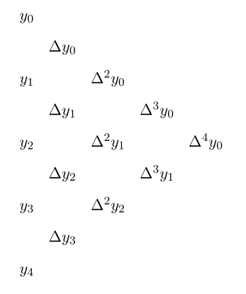
Triangular table with y0 to y4 in the first column, the first finite differences delta y0 to delta y3 in the second column, the second finite differences delta^2 y0 to delta^2y2 in the third column, the third finite differences delta^3 y0 and delta^3 y1 in the fourth column, and the fourth finite difference delta^4 y0 in the last column.

Figure 19.1: Triangular table used to calculate finite differences

Exercise 19.5 Find the \(4\)-th order polynomial which passes through the points \((0,5), (1, 7), (2, 19), (3,54)\), and \((4, 134)\)

Solution. We have \(y_0=5, y_1=7, y_2=19, y_3=54\), and \(y_4=134\).

Our first step is to find the finite differences.

The first finite differences are \[\Delta y_0=y_1-y_0 = 2, \quad \Delta y_1 = y_2-y_1 = 12, \quad \Delta y_2 = y_3-y_2 = 35,\quad\mbox{and}\quad \Delta y_3 = y_4-y_3=80 \]

The second finite differences are \[\Delta^2y_0 = \Delta y_1 -\Delta y_0 = 10, \quad \Delta^2y_1 = \Delta y_2 -\Delta y_1 = 23, \quad \Delta^2y_2 = \Delta y_3 -\Delta y_2=45\]

The third finite differences are \[\Delta^3 y_0 = \Delta^2 y_1-\Delta^2 y_0=13, \quad \Delta^3 y_1 = \Delta^2 y_2- \Delta^2 y_1 = 22\]

The fourth finite difference is \(\Delta^4 y_0 = \Delta^3 y_1 -\Delta ^3 y_0 = 9\)

Plugging the relevant differences into the formula gives \[y=5+2x+5x(x-1)+\frac{13}{6}x(x-1)(x-2)+ \frac{3}{8}x(x-1)(x-2)(x-3)\]

19.3.2 Non-Integer Nodes

Let’s relax our previous assumptions a little by letting \(x_0, x_1, x_2,\ldots\) be any set of equidistant numbers, i.e. \(x_n=x_0+nh\) for \(n=0,1,2,\ldots\) and \(h\) is the distance between each pair of points. Our polynomial interpolation formula generalizes to what’s known as the Newton Forward Difference Formula:

Given \(n+1\) equidistant points \(x_0, x_1, \ldots, x_n\), the \(n\)th order polynomial passing through them is given by \[y= y_0 + \Delta y_0\frac{(x-x_0)}{h}\Delta y_0 + \frac{1}{2!}\Delta^2 y_0 \frac{(x-x_0)(x-x_1)}{h^2}+ \cdots + \frac{1}{n!}\Delta^n y_0 \frac{(x-x_0)(x-x_1)\cdots (x-x_{n-1})}{h^n}\]

Exercise 19.6 Estimate the value of \(f(1.35)\) if \(f(x)\) passes through the points \((1.2, 1),(1.3, 5),(1.4,12), (1.5, 20)\).

Solution. We have \(n=4\), \(h=0.1\), \(x_0=1.2, x_1=1.3, x_2=1.4, x_3=1.5\), \(y_0=1, y_1=5, y_2=12\), and \(y_3=20\).

The first finite differences are \[\Delta y_0 = 4, \quad \Delta y_1 =7, \quad \Delta y_2 = 8\]

The second finite differences are \[\Delta^2 y_0 = 3, \quad \Delta^2 y_1 =1\]

The third finite difference is \[\Delta^3 y_0 = -2\]

Plugging the relevant differences into the formula gives

\[\begin{align*} y &=1+ 4\cdot\frac{x-1.2}{0.1}+ \frac{3}{2}\frac{(x-1.2)(x-1.3)}{0.1^2}-\frac{1}{12}\frac{(x-1.2)(x-1.3)(x-1.4)}{0.1^3}\\ &= 1+ 40(x-1.2)+150(x-1.2)(x-1.3)-\frac{1000}{3}(x-1.2)(x-1.3)(x-1.4) \end{align*}\]

Finally, we input the value \(x=1.35\) to get \(f(1.35)\approx 8.25\)