Lecture 2 Multivariate Limits
Text References: Course notes pp. 1-10 & Rogawski 14.1-14.3
2.1 Recap
Last time, we learned about scalar fields, which are functions \(f:\mathbb{R}^n\to\mathbb{R}\). We practised calculating the value of such functions given various inputs, and used level curves and cross-sections to graph functions of two variables.
Exercise 2.1 Match the graph of the function to its set of level curves.
| Level.Curves | Graph.of.Function |
|---|---|
1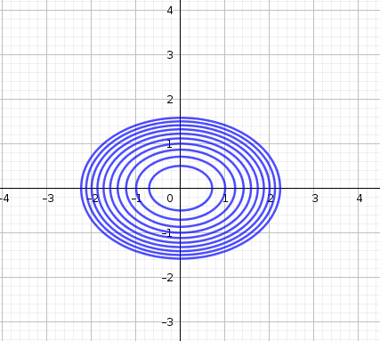 |
a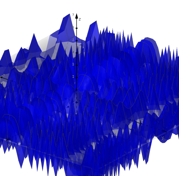 |
2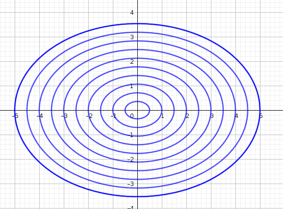 |
b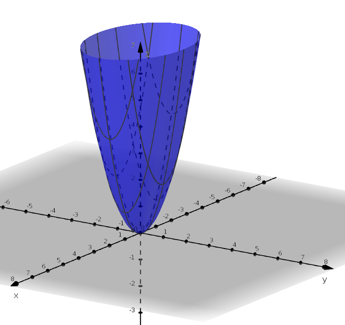 |
3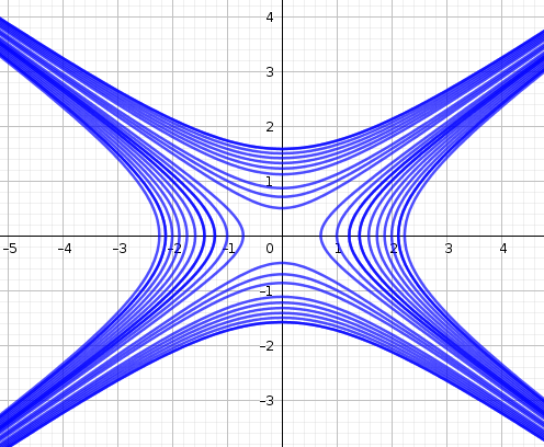 |
c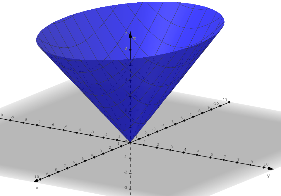 |
4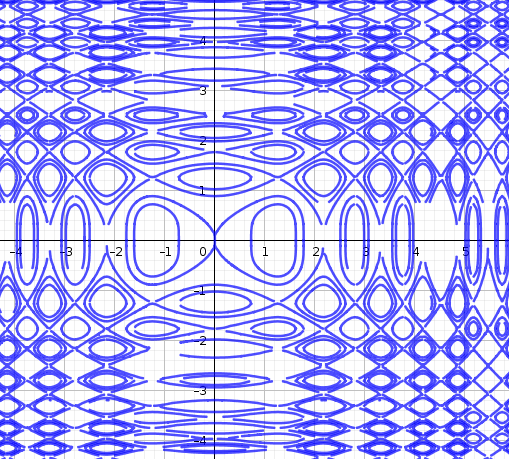 |
d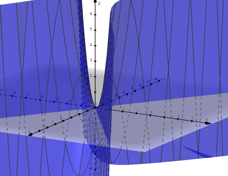 |
Solution. 1 with b, 2 with c, 3 with d, 4 with a. The trickier set is 1/b and 2/c. We tell them apart by observing the spacing between the level curves. The closer the level curves are to each other, the steeper the surface. The paraboloid increases in steepness, so we expect its level curves to get closer and closer together. The cone, on the other hand, ‘opens up’ at a constant rate so its level curves are always evenly spaced apart.
2.2 Learning Objectives
- Given a function of 2 variables, consider different paths of approach.
- Outline how to determine whether the limit of a multivariable function exists.
2.3 Approaching Limit Points
In single-variable calculus, you studied limits of functions. Given a candidate limit point \(a\in\mathbb{R}\), we could approach it either from the left or from the right.
Now, let’s consider a function of two variables \(f:\mathbb{R}^2\to\mathbb{R}\) The domain of \(f\) is the \(xy\)-plane. What are ways in which we can approach a candidate limit point \((a,b)\)?
We notice that there are infinitely many ways to approach \((a,b)\)! As you can imagine, this makes determining the limit of a multivariable function much more difficult since we have infinitely many paths to consider.
Example 2.1 Consider \(\displaystyle \lim_{(x,y)\to(0,0)} \dfrac{2xy}{x^2+y^2}\). Approach \((0,0)\) following three distinct paths and for each path calculate the limit.
- Let’s approach along the path \(y=0\). Then, \(f(x,0)=\dfrac{2(x)(0)}{x^2+0^2}=0\) for \((x,y)\neq (0,0)\). The limit along this path is \(0\).
- Approaching along the path \(x=0\), we have \(f(0,y)=0\) for \((x,y)\neq (0,0)\). The limit along this path is \(0\).
- Approaching along the path \(y=x\), we have \(f(x,x)=\dfrac{2x^2}{2x^2}=1\) for \((x,y)\neq (0,0)\). The limit along this path is \(1\).
See what’s happening in 3D space
Notice that we found different limits when we approached using different paths. As in single-variable calculus, this is an indication that \(\displaystyle \lim_{(x,y)\to(0,0)} \dfrac{2xy}{x^2+y^2}\) does not exist.
2.4 Does the Limit Exist?
We won’t go through the details of calculating limits for multivariable functions in this course. The short version goes like this:
- If we can find (at least) two paths that yield different limit values, then the limit does not exist.
- To prove that the limit does exist, we need to use the Squeeze Theorem.
Exercise 2.2 Consider \(\displaystyle \lim_{(x,y)\to(0,0)} \dfrac{x^3y}{x^6+y^2}\). Find at least two paths of approach that yield different limits. Hint: think about paths that aren’t just straight lines.
Solution. Let’s consider straight lines of the form \(y=mx\) for \(m\in\mathbb{R}\). Note that all of these pass through \((0,0)\) and that the parameter \(m\) allows us to check a family of lines simultaneously.
We have \(f(x,mx) = \dfrac{x^3(mx)}{x^6+(mx)^2} = \dfrac{mx^4}{x^6+m^2x^2}=\dfrac{mx^2}{x^4+m^2}\). As \((x,y)\to(0,0)\), the limit is equal to \(0\).
Now, let’s consider the path \(y=x^3\). Notice that this will give us some nice cancellations in the numerator and the denominator: \(f(x,x^3)=\dfrac{x^3(x^3)}{x^6+(x^3)^2}=\dfrac{x^6}{2x^6}\). As \((x,y)\to(0,0)\), the limit is equal to \(\dfrac{1}{2}\).
We’ve found two paths of approach that yield different limits. Therefore, this limit does not exist.