Lecture 3 Partial Derivatives

Text References: Course notes pp. 1-10 & Rogawski 14.1-14.3

3.1 Recap

Last time, we discussed how we might show that the limit of a multivariable function does not exist.

Exercise 3.1 Show that $\displaystyle \lim_{(x,y)\to(0,0)}\dfrac{x^4-y^5}{x^4+y^4}$ does not exist.

Solution. In order to show that the limit does not exist, we need to find (at least) two paths of approach that give different limit values.

Let’s try the family of straight lines $y=mx$:

We have $\displaystyle \lim_{(x,y)\to(0,0)}\dfrac{x^4-(mx)^5}{x^4+(mx)^4}=\displaystyle \lim_{(x,y)\to(0,0)}\dfrac{x^4(1-m^5x)}{x^4(1+m^4)}=\displaystyle \dfrac{1}{1+m^4}$.

Note that the value of this limit depends on $m$; this means that approaching along different straight lines will give us different limit values and therefore that the limit does not exist.

$3D graph of $f(x,y)=\dfrac{x^4-y^5}{x^4+y^4}$

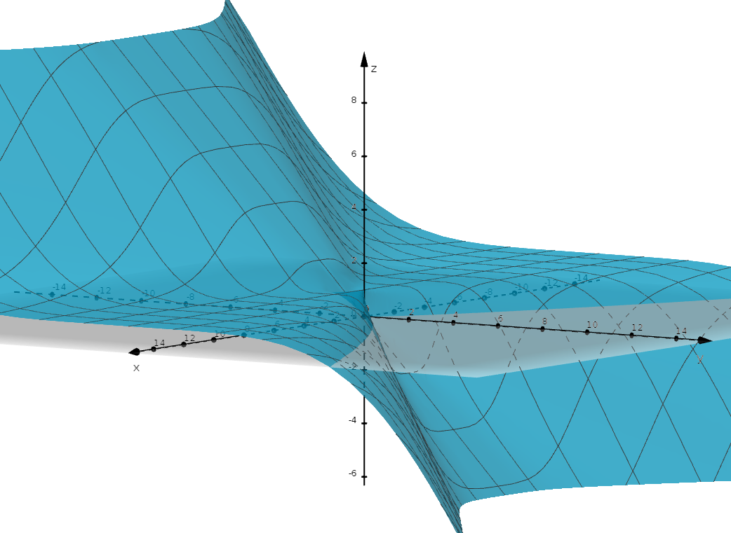
Figure 3.1: Graph of $f(x,y)=\dfrac{x^4-y^5}{x^4+y^4}$

See the following 3D GeoGebra applet which shows the graph of the function.

3.2 Learning Objectives

Given a function of several variables, calculate its first-order partial derivatives.
Given a function of several variables, calculate its higher-order partial derivatives.

3.3 First Order Partial Derivative

Now that we’re dealing with functions of more than one variable, taking derivatives becomes slightly more complicated. Here are the formal definitions:

Definition 3.1 The partial derivative of $f(x,y)$ with respect to $x$ at the point $(a,b)$ is \[f_x(a,b)=\displaystyle \lim_{h\to 0}\dfrac{f(a+h,b)-f(a,b)}{h}\] and the partial derivative of $f(x,y)$ with respect to $y$ at the point $(a,b)$ is \[f_y(a,b)=\displaystyle \lim_{h\to 0}\dfrac{f(a,b+h)-f(a,b)}{h}\] provided that these limits exist.

Notation: You may see a few different notations: $f_x$, $\dfrac{\partial f}{\partial x}$, and $D_1$ are all used to denote the partial derivative of a multivariable function $f$ with respect to $x$ (or, in the case of $D_1$, whichever variable is listed first).

In practice, we only use these definitions when we run into indeterminate forms. Most of the time, however, we can take partial derivatives by holding one variable constant and differentiating with respect to the other.

Exercise 3.2 Calculate the following partial derivatives:

$f_x$ for $f(x,y)=\sin(xy^2)$
$\dfrac{\partial g}{\partial y}$ for $g(x,y,z)=xy^2z^3$
$k_x(0,0)$ for $k(x,y)=(x^3+y^3)^{\frac{1}{3}}$

Solution. We have

Holding $y$ as a constant and differentiating with respect to $x$, we have $f_x = y^2cos(xy^2)$.
Holding $x$ and $z$ as constants and differentiating with respect to $y$, we have $\dfrac{\partial g}{\partial y}= 2xyz^3$.
Holding $y$ as a constant and differentiating with respect to $x$, we have \[k_x(x,y)=\dfrac{x^2}{(x^3+y^3)^{\frac{2}{3}}}\] If we try to evaluate this at $(x,y)=(0,0)$, we have an indeterminate form. This means that we should use the formal definition to calculate this partial derivative:

\[\begin{align*} k_x(0,0)&=\lim_{h\to 0}\dfrac{k(0+h,0)-k(0,0)}{h}\\ &=\lim_{h\to 0}\dfrac{(h^3+0^3)^{\frac{1}{3}}-0}{h}\\&=1 \end{align*}\]

3.4 Higher Order Partial Derivatives

Notice that when we take first-order partial derivatives, we still end up with multivariable functions. We can keep taking partial derivatives for as long as we like! For now, we’ll stick to second-order partial derivatives.

Given a function $f(x,y)$, we found that it had two partial derivatives: $f_x$ and $f_y$. If we take partial derivatives of the partial derivatives, we will end up with four second-order partial derivatives: $f_{xx}$, $f_{xy}$, $f_{yx}$, and $f_{yy}$.

Notation: We have to be a little careful with notation here.

Notation of the form $f_{xy}$ is read from : it means that first, we take the partial derivative w.r.t $x$ and second, we take the partial derivative w.r.t $y$.
Notation of the form $\dfrac{\partial^2 f}{\partial x\partial y}$ is read from : it means that first, we take the partial derivative w.r.t $y$ and second, we take the partial derivative w.r.t $x$.
Notation of the form $D_1D_2f$ is read from from : it means that first, we take the partial derivative w.r.t $y$ and second, we take the partial derivative w.r.t $x$.

Exercise 3.3 Calculate all of the second partial derivatives of $f(x,y)=xe^{2xy}$. What do you notice?

Solution. We have \[ f_x(x,y)=e^{2xy}+2xye^{2xy} \quad \mbox{and} \quad f_y(x,y)=2x^2e^{2xy}\] And therefore \[\begin{align*} f_{xx}(x,y)&=4ye^{2xy}+4xy^2e^{2xy}\\ f_{xy}(x,y)&=4xe^{2xy}+4x^2ye^{2xy}\\ f_{yx}(x,y)&=4xe^{2xy}+4x^2ye^{2xy}\\ f_{yy}(x,y)&=4x^3e^{2xy}\\ \end{align*}\]

We notice that the mixed partial derivatives, $f_{xy}$ and $f_{yx}$ are equal.

A natural question that arises is whether this phenomenon always occurs. Clairaut’s Theorem provides an answer:

Theorem 3.1 (Clairaut's Theorem) If $f_{xy}$ and $f_{yx}$ are defined in some neighbourhood of $(a,b)$ and are both continuous at $(a,b)$, then $f_{xy}(a,b)=f_{yx}(a,b)$.

In this course, the functions that we’ll work with will generally be nice, so this theorem applies. Clairaut’s Theorem also generalizes to higher-order partial derivatives, which is quite handy. One way to use this theorem is to simplify calculations involving mixed partial derivatives.

Exercise 3.4 Let $f(x,y,z,w)=x^3w^2z^2+\sin\left(\dfrac{xy}{z^2} \right)$. Calculate $f_{zzwx}$.

Solution. Note that the second term does not depend on $w$; differentiating first w.r.t $w$ will make this term disappear. Applying Clairaut’s Theorem, we have $f_{zzwx}=f_{wzzx}$.

Taking the partial derivative w.r.t $w$, we have \[f_w = 2x^3wz^2\]

Then, taking the partial derivative w.r.t $z$, we have \[f_{wz}=4x^3wz\]

Taking the partial derivative w.r.t $z$ a second time, we have \[f_{wzz}=4x^3w\]

Finally, taking the partial derivative w.r.t $x$, we have \[f_{wzzx} =12x^2w \]